01 - The training plateau - When the gradient disappears

Quantitative financial data is highly correlated data with an extremely low signal-to-noise ratio. The primary challenge is to extract from an observation window not the sequential sequence of raw values, but the hidden system dynamics - transient pulses, cyclic reversals and energetic state changes. Since these structures are lost in stochastic noise, a standard architecture consumes a disproportionately large part of its capacity for representation formation alone.

If the model hits a plateau, the loss gradient (∇ℒ) collapses. The optimizer loses its directional stability in this flat parameter region because the gradient components converge to zero. At this point, the network has only learned the trivial, dominant variance components. The deeper, predictive structures of the market remain unreached because the current mathematical vocabulary of the network is not sufficient to isolate them cleanly from the noise.

Adaptive optimization methods such as AdamW do not offer a systemic remedy here: they correct the scaling, but cannot extract a direction from a vector field whose expected value is zero on average. Even the conventional reduction of the learning rate(ReduceLROnPlateau) does not break this stagnation. It merely cements it. The network remains in the flat zone and begins to memorize the high-frequency noise structures of the training data - the direct path to overfitting, which causes the validation metric to degrade with a time delay.

The plateau is not the end of learning. It is the end of the current vocabulary.
- Diagnosis of the stagnation problem

02 - The foundation - Koopman: When movement becomes linear algebra

The American mathematician Bernard Koopman published a paper 1931 that hardly anyone needed at the time and has found its way into every textbook on data-driven dynamics in the last ten years. At first glance, his idea is paradoxical: if a system moves in a complicated non-linear way, it can still be described linearly - if you are prepared to switch to an infinite-dimensional space in which it is not the states themselves that develop, but functions over states.

This sounds like a bad trade-off - a finite-dimensional nonlinear problem for an infinite-dimensional linear one. In reality, it is an excellent exchange, because linear operators have something that non-linear functions usually do not: a spectrum. Eigenvalues and eigenvectors. Clear, decomposable building blocks. Anyone who knows the Koopman operator of a system knows its eigenmodes - the fundamental oscillation patterns from which every actual movement is composed, just as every sound can be composed of pure sine tones.

No one can calculate the exact Koopman operator of a market dynamics system. But it is possible to learn a finite-dimensional approximation from data - the method is called Dynamic Mode Decomposition, or DMD for short. In its kernel-based variant, as used by the encoder, a small matrix is automatically obtained from an observation window whose eigenvalues precisely answer two questions: how fast does this dynamic oscillate, and does it gain or lose energy.

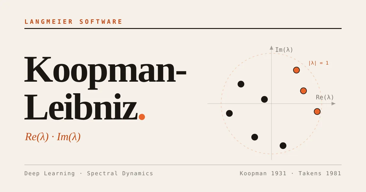
Diagram 01 - What a complex eigenvalue means
Each point in the complex plane is a whole mode of motion - frequency and growth in one number

• Energy-building modes (real part > 0) - orange
• Energy-depleting modes (real part < 0) - dark
• Stability limit - dashed circle

This map is the central visualization needed to understand the encoder. An observation window is mapped to ten points in this complex plane. Each point is an independent type of movement that the system currently contains. The real part tells you whether this movement is picking up speed or coasting; the imaginary part tells you how fast it is oscillating. The entire window can be reconstructed from these ten points, without the detour via several hundred raw numbers.

03 - Spectral reduction - isolating the system primitives

The structural challenge in modeling the Koopman space lies in its numerical unwieldiness: it is infinite-dimensional by construction. The mathematical mastery of this dimensionality draws a direct parallel to Gottfried Wilhelm Leibniz's Characteristica Universalis and his Ars Combinatoria. With the Alphabetum cogitationum humanarum, Leibniz postulated a universal system that traces complex, continuous dynamics back to a finite set of orthogonal, indivisible basic concepts - the notiones primitivae. Complexity is not understood here as a chaotic continuum, but as a linear combination of discrete, primitive building blocks.

Algorithmically, this rational reduction forms the foundation for the rank truncation within the Hilbert space ℋ, which the RBF kernel implicitly spans. While the similarity matrix K₀ encodes the complete, noisy trajectory of the observation window, the subsequent symmetric eigenvalue decomposition isolates the k dominant eigenmodes. This is the formal act of primitive isolation - a projection onto the low-dimensional, Koopman-invariant subspace:

Spectral projection - Leibniz rank reduction

ℋ  ⟶  ?ₖ

ℋ represents the infinite-dimensional Hilbert space as the formal carrier of the entire potential dynamics. ?ₖ defines the k-dimensional subspace spanned by the dominant eigenmodes; in the standard setup, k = 10. All spectral components beyond this boundary are analytically discarded as transient noise.

This truncation operates as the primary regularization mechanism of the encoder. A neural network operating on the unfiltered spectrum inevitably memorizes the high-frequency, stochastic singularities of the training sample. By compressing the signal to the k dominant primitives, the architecture enforces a mathematical abstraction: the downstream layers do not extract the ephemeral noise structures of a specific window, but the invariant generators of the system dynamics.

04 - The machine - From raw signal to spectral fingerprint

What the encoder does internally can be read as six successive stages, each of which solves a specific problem. We go through the central steps mathematically - not as a code walkthrough, but as an argumentation that answers a question in each case.

The first step establishes comparability. The kernel that follows immediately works with distances in an exponential function. If the input values are numerically large, the exponential function collapses to zero and the entire pipeline produces only zeros. Per window is therefore standardized locally.

Local standardization

x̂ = (x − μ) / (σ + ε)

Each value is reduced by the window mean value μ and divided by the window standard deviation σ. The small summand ε prevents division by zero for quiet phases. This makes the encoder level-invariant: a movement of one percent looks the same to it, regardless of the absolute level at which it takes place. The model learns dynamics, not absolute values.

The second step turns history into a state. A single observation says almost nothing. Dynamics is the relationship between successive states. The window is split into two time-delayed versions - the first contains the observations up to the penultimate step, the second the observations from the second step to the end. The transition rule will later be derived from the comparison of these two versions. It is the old Takens idea: progression is state.

The third step is the actual mathematical trick: similarity as geometry. Instead of manually inventing indicators, the encoder lets the geometry of the data speak for itself. For each point in time in the window, it measures how similar it is to all other points in time. The measure of similarity is the RBF kernel:

RBF kernel - the similarity measure

k(x, y) = exp(−γ · ‖x − y‖²)

The expression ‖x - y‖² is the square of the Euclidean distance between two states - how far apart they are in space. The exponential function compresses this to a value between 0 and 1: identical states result in exactly 1, distant states result in practically 0. The parameter γ controls how quickly the similarity decreases with increasing distance - it is, so to speak, the sharpness with which the system separates "similar" from "different".

The window thus becomes a similarity matrix in which each entry is a similarity value between two points in time. This is no longer a time series - it is a topography. Which phases are similar, which are not, and how is this distributed across the window. A second similarity matrix compares each time point with its successor and will carry the information for the transition rule.

The fourth step finds the alphabet: An eigenvalue decomposition is applied to the first similarity matrix. The largest eigenvalues show the dominant patterns of the topography. Here we cut off - only the top-k modes remain, the Leibniz primitives of the window.

The fifth step constructs the transition rule. In the space of dominant modes, a small matrix is built that describes exactly how the window evolves from one time step to the next:

Reduced Koopman matrix in mode space

à = Σ⁻¹ · Vᵀ · K₁ · V · Σ⁻¹

V contains the top-k eigenvectors of the first similarity matrix - the alphabet. K₁ is the time-shifted similarity matrix that encodes the transition from one time step to the next. Σ-¹ normalizes the lengths of the eigenvectors so that the resulting matrix is not distorted by scale differences. What remains is a linear operator on a nonlinearly generated space - Koopman's original idea, here in reduced form.

The sixth and final step reads out the essence. A second eigenvalue decomposition is applied to this small matrix - this time one that allows for complex values. Each mode becomes a complex eigenvalue. Its real part is the growth rate, its imaginary part is the frequency. A window of several hundred raw values thus becomes 2 × k values - i.e. twenty numbers for ten modes, which together carry the entire dynamics of the window.

05 - The implementation - The core that does the math

What is remarkable about the implementation is not its length, but its brevity. What sounds like a specialized lecture in theory is just a few precise lines in PyTorch - without having to write a single loop. The entire spectral apparatus lives in two built-in routines for eigenvalue decompositions. This makes the encoder not only readable - it makes it fully differentiable. It can be built into any neural network as a layer and trained by backpropagation.

# proprietary — interne Implementierung gekürzt
class KoopmanLeibnizEncoder(nn.Module):
    def __init__(self, rank=10, gamma=0.1):
        super().__init__()
        self.rank  = rank     # Anzahl beibehaltener Leibniz-Primitive
        self.gamma = gamma    # Breite des RBF-Kernels

    def forward(self, x):
        # Lokale Standardisierung pro Fenster — gegen Kernel-Kollaps
        x = (x - x.mean(dim=1, keepdim=True)) / (x.std(dim=1, keepdim=True) + 1e-6)

        # [...] Takens-Einbettung, RBF-Kernel, Spektrum, reduzierte Koopman-Matrix
        # [...] interne Pipeline — Details proprietär
        A_tilde = _internal_spectral_pipeline(x, self.rank, self.gamma)

        # Komplexe Eigenwerte → Wachstum (Re) + Frequenz (|Im|)
        koop_vals, _ = torch.linalg.eig(A_tilde)
        return torch.cat([koop_vals.real, torch.abs(koop_vals.imag)], dim=-1)
                              PYTHON
                            

The encoder is therefore not an upstream data tool, but an integral component of the architecture. What it produces is a spectral fingerprint of the observation window: twenty values that summarize the growth, attenuation and frequency of the dominant market modes. How this information finds its way into the model is the really interesting part - and the reason why this article was written in the first place.

06 - The application - the plateau breaker

In the team's research operation, the large main model, a Transformer-based system with specialized output branches and multiple time planes, repeatedly plateaued in Stage 4. The loss fell cleanly over six to eight epochs, then remained flat. Validation metrics rose slightly - the first indication of incipient adaptation to training specifics. Classic antidotes did not work. Lowering learning rate exacerbated symptoms. More data provided slight improvements that were lost in the variance of multiple runs. The problem was structural: the model had extracted everything it could from the local statistical features. What it needed was not another optimization - but new information.

This is where the Koopman-Leibniz encoder comes into play, but in a role for which it was not originally intended. Instead of being the primary encoder in front of the model, it is used as a parallel information channel - a second data pipeline that feeds the global market modes to the already trained model over several time levels. The connection is made via a cross-attention layer: the main model asks the spectral fingerprint for information that it is missing and integrates the answer into its internal representations.

Such an extension in the middle of training is usually risky. An additional branch changes the gradient landscape abruptly. In the worst case, it destabilizes what has been built up over weeks. This is exactly where the second, almost more important component of the experiment comes into play: the zero-init gate.

Diagram 02 - The gate behavior at the plateau
How a gate started at zero opens exactly when the loss gradient disappears

• Phase 1 - Baseline is stable, gate remains closed - no intervention in the existing learning.
• Phase 2 - Loss flattens out, gradients collapse, the gate opens by itself and the spectral channel begins to take effect.

The gate is mathematically a single scalar quantity - we call it α. It is initialized with the value exactly zero and multiplies the contribution of the new spectral channel before it flows back into the main model:

Residual intervention via the gate

h_neu = h_alt + α · CrossAttn(h_alt, z_spektral)

h_alt is the previous internal representation of the main model. z_spectral is the sequence of spectral fingerprints from the Koopman-Leibniz encoder over several time planes. The CrossAttn operation allows the main model to specifically access information from the spectral channel. As long as α = 0, the entire additional term is exactly zero and the model behaves identically to before.

This construction is the theoretical core. The second term on the right-hand side is exactly zero at the beginning - not small, not negligible, but analytically zero. The main model sees no change, continues to run on its previous loss landscape, keeps all weights stable. The only thing that changes is that there is now a parameter α with a defined gradient. If the backpropagation path determines that an increase in α would reduce the loss, then - and only then - will the gate open.

On a plateau, where all other gradients disappear, the gradient with respect to α is typically the only one that still carries a clear signal. The optimizer has no other way to reduce the loss - so it starts to increase α minimally. The spectral channel thus begins to feed information into the main model. The loss landscape, which was just flat, takes on a new direction. The plateau breaks.

As long as the model converges stably, the additional path remains neutral. Only when the gradient stagnates does the spectral channel become an effective update path.
- How the zero-init mechanism works

This construction is mathematically elegant, but two properties make it particularly valuable in a research setting. First, it is a zero-risk extension: as long as the model progresses without help, the extension is ineffective. There is no stability tradeoff, no disruption of ongoing optimization, no new tuning of the training schedules. Secondly, it does not combat the symptom of the plateau, but the cause. Classic methods like ReduceLROnPlateau slow down the movement when it stops working - they do the wrong thing more precisely. The plateau-breaker instead adds fundamentally new information to the model: global market modes across multiple time levels that were not mathematically present in the local input features.

In the wider research canon, this mechanism is related to methods such as ReZero and LayerScale - both work with residual paths whose contribution is controlled by a learnable scaling factor that starts at zero. What distinguishes the Plateau-Breaker is its function: the residual extension does not add depth to the mesh, but a specific class of information - spectral system modes that the encoder explicitly extracts. It is not more model capacity, but a different representation basis.

07 - The punchline - Three properties that work together

Spectral methods in time series analysis are nothing new. What makes the Koopman-Leibniz variant qualitatively new in this combination - encoder plus zero-init-gate plus cross-attention - are three properties that reinforce each other.

It is level-invariant. Due to the local normalization per window, the encoder sees movements, not levels. The model that works with this mechanism can run on any market dynamics system without absolute value ranges ever playing a role.

It is non-linear without having to invent non-linear features. The RBF kernel implicitly embeds the data in an infinite-dimensional space in which complicated non-linear relationships become linear structures. No one has to guess which indicators the system might need - the geometry of the data generates the non-linear relationships itself.

It can be interpreted spectrally. What arrives at the output are not mysterious latent variables, but growth and frequency values with a clear dynamic meaning. If you want to know why a model made a certain decision in a certain situation, you can look at the spectral fingerprint and literally read off the dynamic state the system was in at the time.

Classical scalers normalize numbers. The Koopman-Leibniz encoder normalizes meaning.
- In plain language

There is no semantic difference. Giving a model raw time series forces it to perform the translation into dynamics itself - with the full capacity of its weight matrices and the full effort of training. Giving it the dynamics in advance suddenly frees up capacity that the model can use for actual decisions.

It is the same mechanism behind specialized training auxiliary targets - small side outputs that force the network to explicitly reconstruct relevant quantities in early layers - only one level deeper. Such auxiliary goals force the backbone to understand the world before it decides. The Koopman-Leibniz encoder forces the input data to reveal its dynamics before it even reaches the model. In the plateau-breaker setup, this becomes a third property: the model is allowed to continue learning exactly when it had actually stopped.

08 - Outlook - What comes next

The mathematical tools are all from the classical repertoire - Bernard Koopman 1931, Floris Takens 1981, the RBF kernel from the standard statistical toolbox, residual learning techniques from recent deep learning research. What has changed is the hardware. A few decades ago, eigenvalue decomposition was a serious numerical effort. Today, it is done in a PyTorch forward pass on the GPU in microseconds - and above all differentiable, i.e. embeddable in any gradient-based training pipeline.

This shifts what is considered feature engineering. Instead of choosing indicators by hand or leaving it to the network to come up with its own representations, an entire class of encoders can be built that write mathematical structures - spectral decompositions, topologies, differential operators - directly into the data flow. The Koopman-Leibniz encoder is an instance of this. Combined with zero-init gates, it becomes something that has been missing in common ML practice to date: a tool that does not combat the symptom of stagnant training, but its mathematical cause.

A dividing line is thus emerging that goes beyond the specific application. The dominant AI architectures of today - from the large language models from companies such as OpenAI, Anthropic or Google DeepMind to the latest generative transformers - are anthropocentric at their core (from the Greek ánthropos, "human"): They model human language, human perception, human decision-making, and they are frozen in a learned, discrete parameter space whose geometry they never leave after training. Koopman-Leibniz operators, on the other hand, work in a continuous spectral space of invariant system laws. This opens up a separate field of research beyond the human-centered model class: generative adaptive transformers that do not derive their representation from human data, but from the dynamics of the observed system itself.

Current testing shows that the encoder does not break through the plateau by adding capacity, but by filtering the system dynamics more precisely. It acts as a selective trigger - it remains inactive in phases in which the model converges independently and only intervenes when gradient stagnation threatens. The system thus gains stability without compromising the existing, learned feature vocabulary.

If the network stagnates on the plateau, it no longer lacks input, but the resolution to extract the signal cleanly from the noise.
- Operational principle of the Koopman-Leibniz method